import matplotlib.pyplot as plt
import numpy as np

from fiberpy.orientation import (
    fiber_orientation,
    Shear,
    shear_steady_state,
    Icosphere,
    distribution_function,
)
from scipy import integrate
from matplotlib.tri import Triangulation

params = {
    "figure.figsize": (6, 4),
    "figure.dpi": 72,
    "axes.titlesize": 14,
    "axes.labelsize": 14,
    "font.size": 14,
    "xtick.labelsize": 14,
    "ytick.labelsize": 14,
    "legend.fontsize": 14,
    "savefig.bbox": "tight",
    "figure.constrained_layout.use": True,
}
plt.rcParams.update(params)
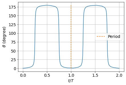
Jeffery’s equation#
ar = 25
gamma = 1
L = np.array([[0, gamma], [0, 0]])
T = 2 * np.pi / gamma * (ar + 1 / ar)
phi0 = [
    1e-4,
]


def dphi(t, phi):
    return ar**2 / (1 + ar**2) * (
        -np.sin(phi) * np.cos(phi) * L[0, 0]
        - np.sin(phi) ** 2 * L[0, 1]
        + np.cos(phi) ** 2 * L[1, 0]
        + np.sin(phi) * np.cos(phi) * L[1, 1]
    ) - 1 / (1 + ar**2) * (
        -np.sin(phi) * np.cos(phi) * L[0, 0]
        + np.cos(phi) ** 2 * L[0, 1]
        - np.sin(phi) ** 2 * L[1, 0]
        + np.sin(phi) * np.cos(phi) * L[1, 1]
    )


sol = integrate.solve_ivp(dphi, (0, 2 * T), phi0, method="Radau")
sol.y = np.abs((sol.y + np.pi) % (2 * np.pi) - np.pi)

plt.plot(sol.t / T, np.rad2deg(sol.y[0, :]))
plt.plot([1, 1], [0, 180], "--", label="Period")
plt.xlabel("$t/T$")
plt.ylabel(r"$\theta$ (degree)")
plt.grid()
plt.legend()

plt.show()
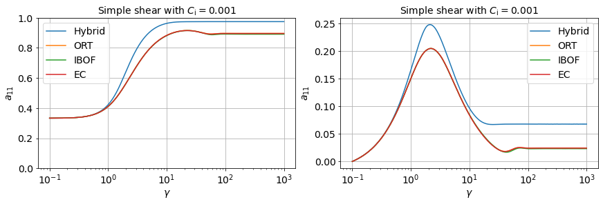
Folgar-Tucker#
ci = 1e-3
ar = 25
t = np.logspace(-1, 3, 1000)
a0 = np.eye(3) / 3

fig, ax = plt.subplots(1, 2, figsize=(12, 4))
a = fiber_orientation(a0, t, Shear, ci, ar, closure="hybrid")
ax[0].semilogx(t, a[0, :], "-", label="Hybrid")
ax[1].semilogx(t, a[2, :], "-", label="Hybrid")

a = fiber_orientation(a0, t, Shear, ci, ar, closure="orthotropic")
ax[0].semilogx(t, a[0, :], "-", label="ORT")
ax[1].semilogx(t, a[2, :], "-", label="ORT")

a = fiber_orientation(a0, t, Shear, ci, ar, closure="invariants")
ax[0].semilogx(t, a[0, :], "-", label="IBOF")
ax[1].semilogx(t, a[2, :], "-", label="IBOF")

a = fiber_orientation(a0, t, Shear, ci, ar, closure="exact")
ax[0].semilogx(t, a[0, :], "-", label="EC")
ax[1].semilogx(t, a[2, :], "-", label="EC")

ax[0].set_xlabel(r"$\gamma$")
ax[1].set_xlabel(r"$\gamma$")
ax[0].set_ylabel("$a_{11}$")
ax[1].set_ylabel("$a_{11}$")
ax[0].set_title(r"Simple shear with $C_\mathrm{i}=%g$" % ci)
ax[1].set_title(r"Simple shear with $C_\mathrm{i}=%g$" % ci)
ax[0].grid()
ax[1].grid()
ax[0].set_ylim(0, 1)
ax[0].legend()
ax[1].legend()

fig.show()
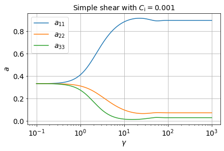
ci = 1e-3
ar = 25
t = np.logspace(-1, 3, 1000)
a0 = np.eye(3) / 3

a = fiber_orientation(a0, t, Shear, ci, ar, closure="orthotropic")
plt.semilogx(t, a[0, :], "-", label="$a_{11}$")
plt.semilogx(t, a[4, :], "-", label="$a_{22}$")
plt.semilogx(t, a[8, :], "-", label="$a_{33}$")

plt.xlabel(r"$\gamma$")
plt.ylabel("$a$")
plt.title(r"Simple shear with $C_\mathrm{i}=%g$" % ci)
plt.grid()
plt.legend()
plt.show()
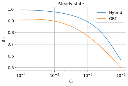
ar = 25
ci = np.logspace(-4, -1, 50)
a_hybrid = np.zeros((len(ci), 9))
a_orthotropic = np.zeros((len(ci), 9))

for i in range(len(ci)):
    a_hybrid[i, :] = shear_steady_state(ci[i], ar, closure="hybrid")
    a_orthotropic[i, :] = shear_steady_state(ci[i], ar, closure="orthotropic")

plt.semilogx(ci, a_hybrid[:, 0], "-", label="Hybrid")
plt.semilogx(ci, a_orthotropic[:, 0], "-", label="ORT")

plt.xlabel(r"$C_\mathrm{i}$")
plt.ylabel(r"$a_{11}$")
plt.grid()
plt.title("Steady state")
plt.legend()

plt.show()
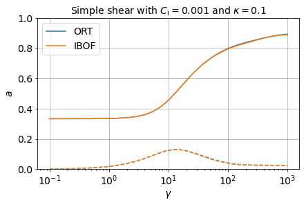
RSC model#
ci = 1e-3
kappa = 0.1
ar = 25
t = np.logspace(-1, 3, 1000)
a0 = np.eye(3) / 3

a = fiber_orientation(a0, t, Shear, ci, ar, kappa, closure="orthotropic")
plt.semilogx(t, a[0, :], "C0-", label="ORT")
plt.semilogx(t, a[2, :], "C0--")

a = fiber_orientation(a0, t, Shear, ci, ar, kappa, closure="invariants")
plt.semilogx(t, a[0, :], "C1-", label="IBOF")
plt.semilogx(t, a[2, :], "C1--")

plt.xlabel(r"$\gamma$")
plt.ylabel("$a$")
plt.title(r"Simple shear with $C_\mathrm{i}=%g$ and $\kappa=%g$" % (ci, kappa))
plt.grid()
plt.ylim(0, 1)
plt.legend()
plt.show()
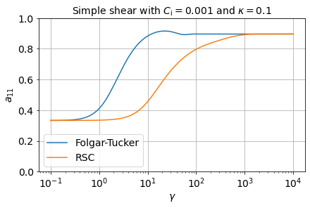
ci = 1e-3
ar = 25
t = np.logspace(-1, 4, 1000)
a0 = np.eye(3) / 3

a = fiber_orientation(a0, t, Shear, ci, ar)
plt.semilogx(t, a[0, :], "-", label="Folgar-Tucker")

kappa = 0.1
a = fiber_orientation(a0, t, Shear, ci, ar, kappa)
plt.semilogx(t, a[0, :], "-", label="RSC")

plt.xlabel(r"$\gamma$")
plt.ylabel("$a_{11}$")
plt.title(r"Simple shear with $C_\mathrm{i}=%g$ and $\kappa=%g$" % (ci, kappa))
plt.grid()
plt.ylim(0, 1)
plt.legend()
plt.show()
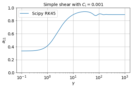
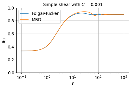
MRD model#
ci = 1e-3
ar = 25
t = np.logspace(-1, 3, 1000)
a0 = np.eye(3) / 3

D3 = (1, 0.5, 0.3)
a = fiber_orientation(a0, t, Shear, ci, ar, D3=D3)
plt.semilogx(t, a[0, :], "-", label="Scipy RK45")

# a = fiber_orientation(a0, t, Shear, ci, ar, D3=D3, method="julia")
# plt.semilogx(t, a[0, :], "-", label="Julia")

plt.xlabel(r"$\gamma$")
plt.ylabel("$a_{11}$")
plt.title(r"Simple shear with $C_\mathrm{i}=%g$" % ci)
plt.grid()
plt.ylim(0, 1)
plt.legend()
plt.show()
ci = 1e-3
ar = 25
t = np.logspace(-1, 3, 1000)
a0 = np.eye(3) / 3

sol, dadt_FT = fiber_orientation(a0, t, Shear, ci, ar, debug=True)
plt.semilogx(t, sol.y[0, :], "-", label="Folgar-Tucker")

D3 = (1, 0.5, 0.3)
sol, dadt_MRD = fiber_orientation(a0, t, Shear, ci, ar, D3=D3, debug=True)
plt.semilogx(t, sol.y[0, :], "-", label="MRD")

plt.xlabel(r"$\gamma$")
plt.ylabel("$a_{11}$")
plt.title(r"Simple shear with $C_\mathrm{i}=%g$" % ci)
plt.grid()
plt.ylim(0, 1)
plt.legend()
plt.show()
Orientation distribution function#
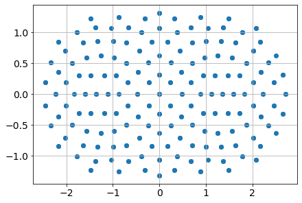
Equal Earth projection#
A projection of sphere surface to 2-d plane, see https://en.wikipedia.org/wiki/Equal_Earth_projection.
icosphere = Icosphere(n_refinement=2)
x, y = icosphere.equal_earth_projection()

plt.scatter(x, y)
plt.grid()
plt.show()
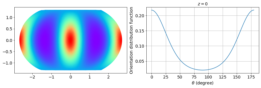
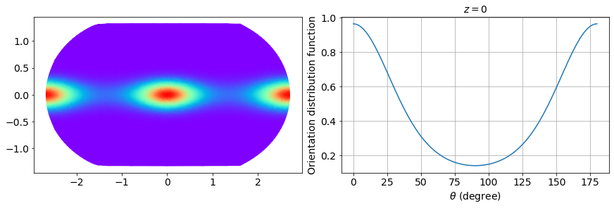
Reconstruction of fiber orientation distribution function#
ODF, mesh = distribution_function([0.7, 0.28, 0.02], n_refinement=5, return_mesh=True)
x, y = mesh.equal_earth_projection()
tri = Triangulation(x, y)

plt.figure(figsize=(12, 4))
plt.subplot(1, 2, 1)
plt.tripcolor(tri, mesh.point_data["ODF (points)"], cmap="rainbow", shading="gouraud")

plt.subplot(1, 2, 2)
theta = np.linspace(0, np.pi, 100)
x = np.vstack([np.cos(theta), np.sin(theta), np.zeros_like(theta)]).T
p = ODF(x)
plt.plot(np.rad2deg(theta), p)
plt.xlabel(r"$\theta$ (degree)")
plt.ylabel("Orientation distribution function")
plt.title("$z=0$")
plt.grid()
plt.show()

# meshio.write("test.vtu", mesh)
ODF, mesh = distribution_function([0.5, 0.2, 0.3], n_refinement=5, return_mesh=True)
x, y = mesh.equal_earth_projection()
tri = Triangulation(x, y)

plt.figure(figsize=(12, 4))
plt.subplot(1, 2, 1)
plt.tripcolor(tri, mesh.point_data["ODF (points)"], cmap="rainbow", shading="gouraud")

plt.subplot(1, 2, 2)
theta = np.linspace(0, np.pi, 100)
x = np.vstack([np.cos(theta), np.sin(theta), np.zeros_like(theta)]).T
p = ODF(x)
plt.plot(np.rad2deg(theta), p)
plt.xlabel(r"$\theta$ (degree)")
plt.ylabel("Orientation distribution function")
plt.title("$z=0$")
plt.grid()
plt.show()

# meshio.write("test2.vtu", mesh)